Integration of Physical Observation Components by Spherical Cap Harmonics Parametrization: 2nd stage of the DFHRS Concept and Software (Version 5.0)

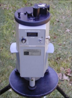
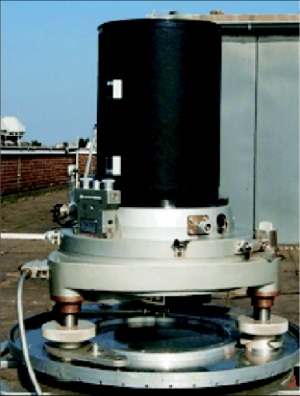
The extension of DFHRS concept and software to physical observation types - such as terrestrial, air- or space-borne gravity measurements (for terrestrial gravity meter see fig. 3), or physical observation types taken from geopotential models (GPMs), e.g. EGM 2008 - is based on a regional spherical cap harmonic parameterization (SCH) of the Earth’s gravitational potential (V).

The benefit of an SCH-parameterization (3) with a local cap pole and a limited cap size area, instead of an ordinary global spherical harmonic (SH), is that the same resolution of V can be achieved with SCH by a much smaller number of parameters than with SH. Thus, for a 2 mm resolution for the HRS, a degree of 7200 for the SH parameterization by (C_n,m,S_n,m) is required, while for a cap size area of 100 km a degree of only k_max=80 is enough in the case of an SCH parametric model. Therefore, SCH is the key model for enabling the computation of high resolution HRS in the 2nd stage of the DFHRS research and development, meaning an integrated over-determined HRS-computation for all types of geometrical and physical observations. The representation of gravitational potential V of the Earth in terms of SCH with parameters (C'_n(k),m,S'_n(k),m) reads:

\begin{array}{l} V(r,\lambda ',\theta ')= \sum\limits_{k=0}^{k\max }\left( \frac{a}{r} \right) ^{n(k)+1} \sum\limits_{m=0}^{k}(C'_{n(k),m} \cdot \cos m\lambda '+S'_{n(k),m'} \cdot \sin m\lambda ')\cdot P'_{n(k),m} (\cos \theta ') \end{array}

(3)

Here the space position refers to the triple of spherical cap coordinates (r, λ', θ' ). In the following, the observation equation for terrestrial and air- or space-borne gravity observations g_p is briefly worked out.
The gravity observation g_p at the Earth surface point P (taken with a gravity meter, see fig. 3, left) is referring to the local astronomical vertical (LAV) system, and, therefore, for the respective observed 3D gravity vector we have in total:

\mathbf{g}^{LAV} =\lbrack 0,0,-g_{P} ]^{T}

Original gravity observation and vector

(4a)

The astronomical vertical (Φ=B+ξ, Λ=L+η/cos(B)) is set up by the ellipsoidal vertical (B, L) and the deflections - from the vertical (ξ,η). The original vector g^LAV (4a) is first rotated to the Earth-centred Earth-fixed system (ECEF) using the astronomical direction (Φ,Λ) from a geopotential model. In that coordinate frame, the centrifugal part of g^LAV (4a) is removed, and so the original observation (4a) is strictly reduced with respect to the vertical deflections (“topography”) and the centrifugal acceleration. We thus arrive at:

\mathbf{g}_{red}^{LGV} =\lbrack g_{N} ,g_{E} ,g_{r} ]^{T}

Reduced gravity observation vector.

(4b)

The observation vector

(4b) is then further rotated as to the SCH-representation frame (3). The SCH-related representation of the gravity vector (4b) reads:

\mathbf{g}_{grav}^{SCH} =\lbrack \frac{1}{r} \cdot \frac{\partial V}{\partial \theta '} ,\frac{1}{r\cdot \sin \theta '} \cdot \frac{\partial V}{\partial \lambda } ,\frac{\partial V}{\partial r} ]^{T}

(4c - 1)

The principal component of the reduced observed gravity observation

(4b) is related to the third component of (4c), and the accuracy of the vertical component of the SCH-transformed observation vector (4b) is nearly unaffected by the above reductions. So in the so-called integrated DFHRS approach we have the following observation equation for a gravity observation:

\begin{array}{l} g_{grav_{r}}^{SCH} +v_{g} = \frac{GM}{{r}^{2}} \cdot \sum\limits_{k=0}^{k\max}\left( \frac{a}{r} \right) ^{n(k)+1} (n(k)+1) \cdot \sum\limits_{m=0}^{k}(C'_{n(k),m} \cdot \cos m\lambda '+S'_{n(k),m'} \cdot \sin m\lambda ')\cdot P'_{n(k),m} (\cos \theta ') \end{array}

(4c - 2)

With v_g (4d) we describe the observation correction of the gravity observation in the integrated adjustment approach. By introducing the disturbance potential

applied to the Bruns theorem and Molodenski’s theory, we obtain the observation equation for fitting-points (h – H) converted to quasi-geoid heights (see (5a) below) and vertical deflections (ξ,η)_p (5b, 5c) observed at point P as:

h-N_{Normal} =N_{QG} =\frac{(V-V_{ref} )_{P} }{\gamma _{Q} } =\frac{T_{P} }{\gamma _{Q} }	(5a)
\xi =-\frac{\partial N_{QG} }{\partial B} \cdot \frac{\partial B}{\partial s_{N} } =-\frac{\partial B}{\partial s} \cdot \frac{\partial N_{QG} }{\partial B} =\frac{-1}{(M+h)} \cdot \frac{1}{\gamma _{Q} } \cdot \frac{\partial }{\partial B} T_{p} =\frac{-1}{\gamma _{Q} \cdot (M+h)} \cdot (\frac{\partial T}{\partial B} )_{P}	(5b)
\eta =-\frac{\partial L}{\partial s} \cdot \frac{\partial N_{QG} }{\partial L} =\frac{-1}{(N+h)\cdot \cos B} \cdot \frac{1}{\gamma _{Q} } \cdot \frac{\partial }{\partial L} T_{P} =\frac{-1}{\gamma _{Q} \cdot (N+h)\cdot \cos B} \cdot (\frac{\partial T}{\partial L} )_{P}	(5c)

In a new adjustment-based approach has been reported, which enables estimation of coefficients (C'_n(k),m, S'_n(k),m) for regional SCH model V (3) as functions of coefficients (C_n,m, S_n,m) of a global geopotential model, e.g. EGM-2008. The estimated coefficients (C'_n(k),m, S'_n(k),m) can be introduced as so-called direct observations in the integrated approach, and we thus have:

C'_{n(k),m} +v=\hat{C}

and

S'_{n(k),m} +v=\hat{S}

(6)

The integrated DFHRS approach, represented by eqs. (3-6), is a far reaching alternative to the model described by (2a) to (2f)), because it allows both “geometrical” and “physical” observations. The integrated approach is presently being investigated and implemented in the DFHRS software version 5.0.
Formula (5a) is used to derive the QGeoid NQG from the estimated SCH-parameters. The QGeoid model NQG or a grid (computed by the DFHRS approaches (1–2f) or (3–6), respectively) can be transformed to a Geoid-model by the equation:

N_{G} =N_{QG} +\frac{\bar{g}-\bar{\gamma} }{\bar{\gamma}}\cdot H

(7)

The mean true gravity along the plumbline shown in fig. 1 can be taken from a density model or a geopotential model, while the mean reference gravity value - from the closed formulas related to the GRS80.

Concept