Geometrical Observation Components and Parameterization: 1st development stage of DFHRS Concept and Software (Version 4)

In the DFHRS concept at its first stage of development, a continuous polynomial surface over of a grid of finite element meshes (FEM) with polynomial parameters p (fig. 2a, thin blue lines) is used as a carrier function for the HRS. The FEM surface of the HRS is therefore called NFEM(p|B,L,h), (fig. 2b). For some old height systems H a scale-difference factor Δm has to be considered in addition, so that the DFHRS-model of N (fig. 2a) consists of two parts. The principle of a GNSS-based height determination H (fig. 2) requires submitting the GNSS-height h to the DFHRS(B,L,h)-correction N, reading:

The DFHRS height N = DFHRS(B,L,h) is provided by means of a database (DFHRS_DB), which contains the HRS parameters (p, Δm) together with the mesh-design (fig. 2a) information. DFHRS_DB have become an industrial and user standard for all GNSS-receiver types worldwide, and can also be used for the set-up of new RTCM-transformation messages. In the 1st development stage of the DFHRS approach, geoid- or geopotential model (GPM)-based non-fitted Geoid or QGeoid/geoid heights N, observed astronomical or GPM-based deflections of the vertical (x,h) in any number of groups, and fitting points (B,L,h|H), fig. 2a) were exclusively used as observation groups in a common least squares computation for evaluation of the DFHRS_DB parameters p and Δm. The mathematical model for these observations is given by formulas (2a–f) below. In the case of an adequate stochastic model, the use of gravity-based geoid or quasi-geoid-models N (2b) computed from Stokes-based models or from GPMs, together with the covariance information, is equivalent to the use of the original observed gravity values g. The mathematical model for computation of the DFHRS_DB parameters (p, Δm) using the above so-called geometrical part of observation components reads:

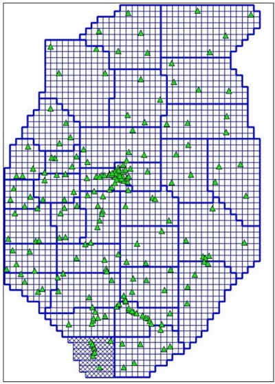
Fig. 2a: Computation design of DFHRS_DB: FEM-Meshes (thin blue lines), patches (thick blue lines) and fitting points (B,L,h|H) (green triangles).

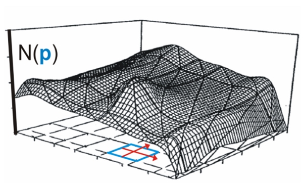
Fig. 2b: HRS polynomials N(p) in single meshes (see also fig. 2a) and as part of a continuous HRS in an arbitrary large area..

By B and L the geodetic latitude and longitude are described. The (x,y) are the projected coordinates. With f_B and f_L we introduce the partial derivatives of f(x(B,L), y(B,L)) (2c) with respect to the geographical coordinates B and L, while M(B) and N(B) mean the radius of meridian and normal curvature, respectively, at a latitude B. The continuity of the resulting HRS representation NFEM(p|x,y) = f(x,y)^Tp over the meshes (fig. 2a, thin blue lines) is automatically provided by the continuity equations C(p) (2f).
A number of identical fitting-points (B,L,h|H) shown in fig. 2 by green triangles are introduced by the observation (Eqs. (2a) and (2e)). In the practice of DFHRS_DB evaluation, one geoid-model a number of different such models - e.g. the EGM 2008 or, in Europe, the EGG97 - are used in the least squares estimation related to the mathematical model (2a–f), which is implemented in the DFHRS-software 4.3. To reduce the effect of medium- or long-wave systematic shape deflections, namely, the natural and stochastic “weak-shapes”, in the observations N and (x,h) from geoid-model (GPM) these observations are subdivided into a number of patches (fig. 2, thick blue lines). These patches are related to a set of individual parameters introduced by the datum parameterizations δN_G(d^j) (2b) and δη(d^j_ξ,η) (2c,d). In this way, it is obviously possible to introduce geoid height observations and vertical deflecttions from any number of different geoid-models (e.g. the EGM 2008) in the same area, or vertical deflections (ξ,η)_P observed with modern zenith cameras (fig. 3, right).

Concept